

On this article, you’ll find out how vector databases work, from the essential thought of similarity search to the indexing methods that make large-scale retrieval sensible.
Matters we are going to cowl embody:
- How embeddings flip unstructured information into vectors that may be searched by similarity.
- How vector databases help nearest neighbor search, metadata filtering, and hybrid retrieval.
- How indexing strategies similar to HNSW, IVF, and PQ assist vector search scale in manufacturing.
Let’s not waste any extra time.
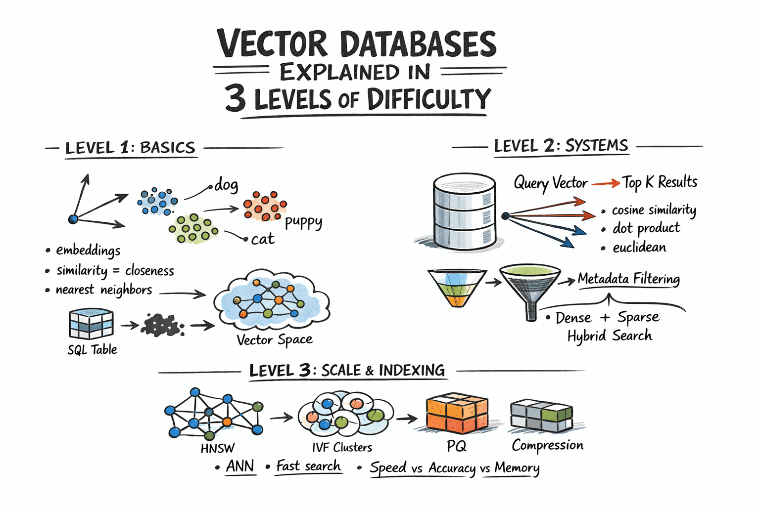
Vector Databases Defined in 3 Ranges of Issue
Picture by Writer
Introduction
Conventional databases reply a well-defined query: does the document matching these standards exist? Vector databases reply a special one: which data are most just like this? This shift issues as a result of an enormous class of recent information — paperwork, photographs, consumer habits, audio — can’t be searched by actual match. So the precise question isn’t “discover this,” however “discover what’s near this.” Embedding fashions make this potential by changing uncooked content material into vectors, the place geometric proximity corresponds to semantic similarity.
The issue, nonetheless, is scale. Evaluating a question vector in opposition to each saved vector means billions of floating-point operations at manufacturing information sizes, and that math makes real-time search impractical. Vector databases clear up this with approximate nearest neighbor algorithms that skip the overwhelming majority of candidates and nonetheless return outcomes practically an identical to an exhaustive search, at a fraction of the associated fee.
This text explains how that works at three ranges: the core similarity drawback and what vectors allow, how manufacturing programs retailer and question embeddings with filtering and hybrid search, and at last the indexing algorithms and structure selections that make all of it work at scale.
Degree 1: Understanding the Similarity Drawback
Conventional databases retailer structured information — rows, columns, integers, strings — and retrieve it with actual lookups or vary queries. SQL is quick and exact for this. However loads of real-world information isn’t structured. Textual content paperwork, photographs, audio, and consumer habits logs don’t match neatly into columns, and “actual match” is the fallacious question for them.
The answer is to symbolize this information as vectors: fixed-length arrays of floating-point numbers. An embedding mannequin like OpenAI’s text-embedding-3-small, or a imaginative and prescient mannequin for photographs, converts uncooked content material right into a vector that captures its semantic that means. Comparable content material produces related vectors. For instance, the phrase “canine” and the phrase “pet” find yourself geometrically shut in vector area. A photograph of a cat and a drawing of a cat additionally find yourself shut.
A vector database shops these embeddings and allows you to search by similarity: “discover me the ten vectors closest to this question vector.” That is known as nearest neighbor search.
Degree 2: Storing and Querying Vectors
Embeddings
Earlier than a vector database can do something, content material must be transformed into vectors. That is completed by embedding fashions — neural networks that map enter right into a dense vector area, usually with 256 to 4096 dimensions relying on the mannequin. The particular numbers within the vector would not have direct interpretations; what issues is the geometry: shut vectors imply related content material.
You name an embedding API or run a mannequin your self, get again an array of floats, and retailer that array alongside your doc metadata.
Distance Metrics
Similarity is measured as geometric distance between vectors. Three metrics are frequent:
- Cosine similarity measures the angle between two vectors, ignoring magnitude. It’s typically used for textual content embeddings, the place path issues greater than size.
- Euclidean distance measures straight-line distance in vector area. It’s helpful when magnitude carries that means.
- Dot product is quick and works properly when vectors are normalized. Many embedding fashions are skilled to make use of it.
The selection of metric ought to match how your embedding mannequin was skilled. Utilizing the fallacious metric degrades end result high quality.
The Nearest Neighbor Drawback
Discovering actual nearest neighbors is trivial in small datasets: compute the gap from the question to each vector, kind the outcomes, and return the highest Ok. That is known as brute-force or flat search, and it’s 100% correct. It additionally scales linearly with dataset measurement. At 10 million vectors with 1536 dimensions every, a flat search is just too sluggish for real-time queries.
The answer is approximate nearest neighbor (ANN) algorithms. These commerce a small quantity of accuracy for giant beneficial properties in pace. Manufacturing vector databases run ANN algorithms below the hood. The particular algorithms, their parameters, and their tradeoffs are what we are going to study within the subsequent degree.
Metadata Filtering
Pure vector search returns probably the most semantically related objects globally. In observe, you often need one thing nearer to: “discover probably the most related paperwork that belong to this consumer and had been created after this date.” That’s hybrid retrieval: vector similarity mixed with attribute filters.
Implementations differ. Pre-filtering applies the attribute filter first, then runs ANN on the remaining subset. Submit-filtering runs ANN first, then filters the outcomes. Pre-filtering is extra correct however dearer for selective queries. Most manufacturing databases use some variant of pre-filtering with sensible indexing to maintain it quick.
Hybrid Search: Dense + Sparse
Pure dense vector search can miss keyword-level precision. A question for “GPT-5 launch date” would possibly semantically drift towards common AI subjects reasonably than the precise doc containing the precise phrase. Hybrid search combines dense ANN with sparse retrieval (BM25 or TF-IDF) to get semantic understanding and key phrase precision collectively.
The usual strategy is to run dense and sparse search in parallel, then mix scores utilizing reciprocal rank fusion (RRF) — a rank-based merging algorithm that doesn’t require rating normalization. Most manufacturing programs now help hybrid search natively.
Degree 3: Indexing for Scale
Approximate Nearest Neighbor Algorithms
The three most necessary approximate nearest neighbor algorithms every occupy a special level on the tradeoff floor between pace, reminiscence utilization, and recall.
Hierarchical navigable small world (HNSW) builds a multi-layer graph the place every vector is a node, with edges connecting related neighbors. Greater layers are sparse and allow quick long-range traversal; decrease layers are denser for exact native search. At question time, the algorithm hops by way of this graph towards the closest neighbors. HNSW is quick, memory-hungry, and delivers wonderful recall. It’s the default in lots of trendy programs.
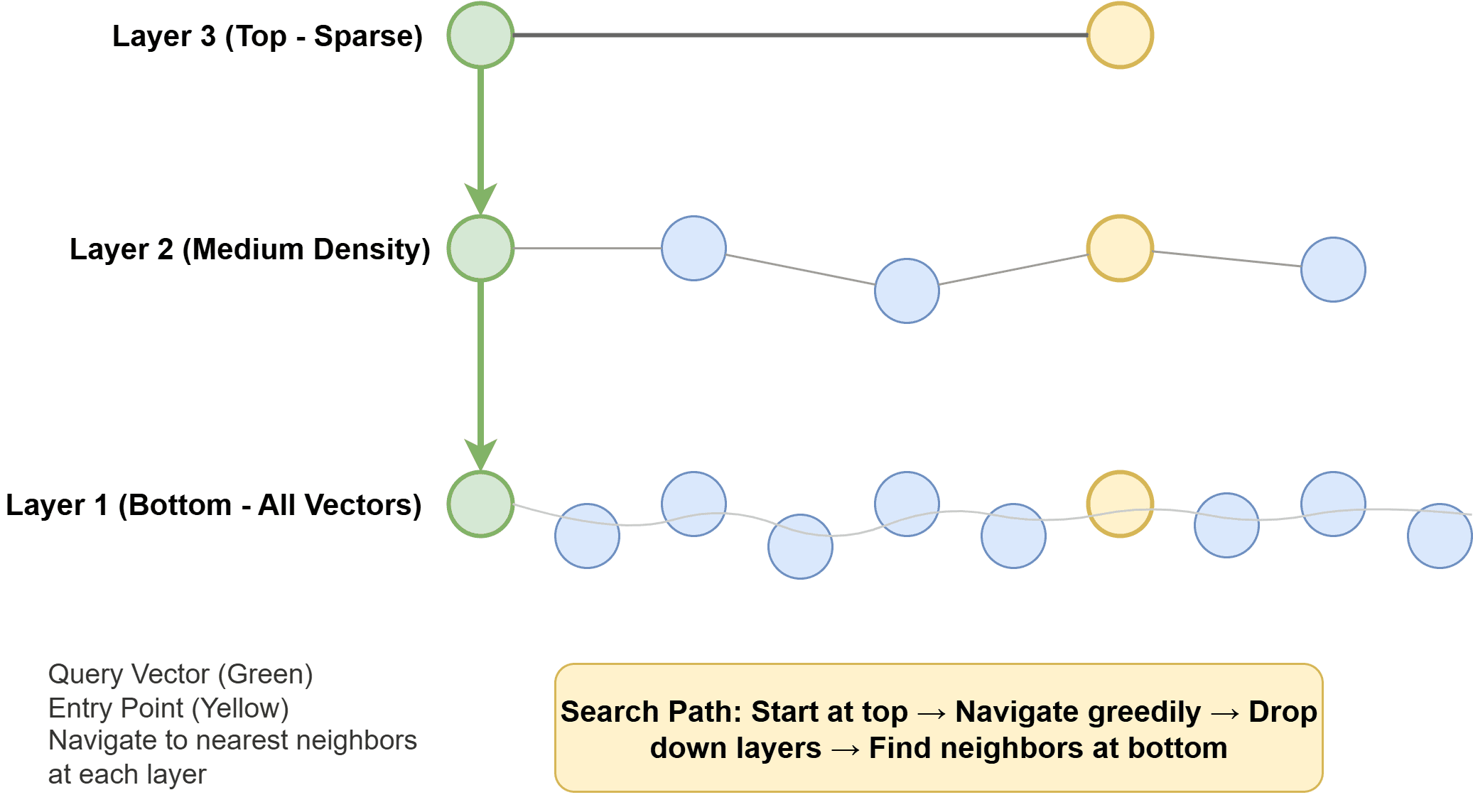
How Hierarchical Navigable Small World Works
Inverted file index (IVF) clusters vectors into teams utilizing k-means, builds an inverted index that maps every cluster to its members, after which searches solely the closest clusters at question time. IVF makes use of much less reminiscence than HNSW however is commonly considerably slower and requires a coaching step to construct the clusters.
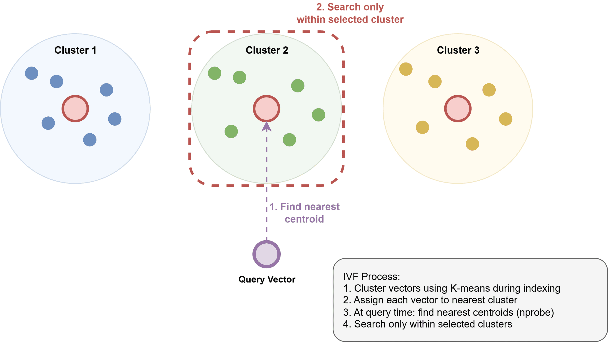
How Inverted File Index Works
Product Quantization (PQ) compresses vectors by dividing them into subvectors and quantizing each to a codebook. This will scale back reminiscence use by 4–32x, enabling billion-scale datasets. It’s typically utilized in mixture with IVF as IVF-PQ in programs like Faiss.
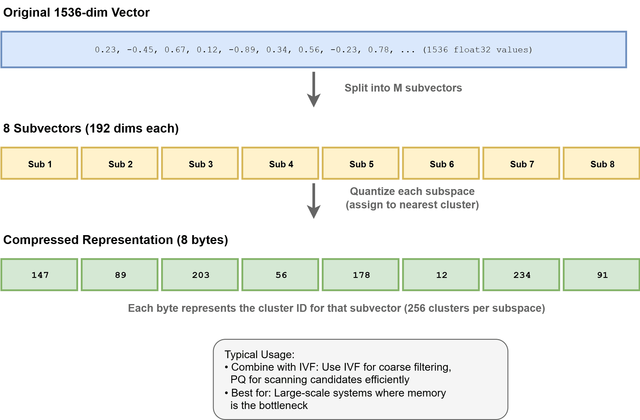
How Product Quantization Works
Index Configuration
HNSW has two important parameters: ef_construction and M:
ef_constructioncontrols what number of neighbors are thought-about throughout index development. Greater values usually enhance recall however take longer to construct.Mcontrols the variety of bi-directional hyperlinks per node. GreaterMoften improves recall however will increase reminiscence utilization.
You tune these based mostly in your recall, latency, and reminiscence finances.
At question time, ef_search controls what number of candidates are explored. Rising it improves recall at the price of latency. This can be a runtime parameter you possibly can tune with out rebuilding the index.
For IVF, nlist units the variety of clusters, and nprobe units what number of clusters to look at question time. Extra clusters can enhance precision but additionally require extra reminiscence. Greater nprobe improves recall however will increase latency. Learn How can the parameters of an IVF index (just like the variety of clusters nlist and the variety of probes nprobe) be tuned to realize a goal recall on the quickest potential question pace? to study extra.
Recall vs. Latency
ANN lives on a tradeoff floor. You possibly can at all times get higher recall by looking out extra of the index, however you pay for it in latency and compute. Benchmark your particular dataset and question patterns. A recall@10 of 0.95 is likely to be nice for a search software; a advice system would possibly want 0.99.
Scale and Sharding
A single HNSW index can slot in reminiscence on one machine as much as roughly 50–100 million vectors, relying on dimensionality and obtainable RAM. Past that, you shard: partition the vector area throughout nodes and fan out queries throughout shards, then merge the outcomes. This introduces coordination overhead and requires cautious shard-key choice to keep away from scorching spots. To study extra, learn How does vector search scale with information measurement?
Storage Backends
Vectors are sometimes saved in RAM for quick ANN search. Metadata is often saved individually, typically in a key-value or columnar retailer. Some programs help memory-mapped information to index datasets which are bigger than RAM, spilling to disk when wanted. This trades some latency for scale.
On-disk ANN indexes like DiskANN (developed by Microsoft) are designed to run from SSDs with minimal RAM. They obtain good recall and throughput for very massive datasets the place reminiscence is the binding constraint.
Vector Database Choices
Vector search instruments usually fall into three classes.
First, you possibly can select from purpose-built vector databases similar to:
- Pinecone: a totally managed, no-operations resolution
- Qdrant: an open-source, Rust-based system with robust filtering capabilities
- Weaviate: an open-source possibility with built-in schema and modular options
- Milvus: a high-performance, open-source vector database designed for large-scale similarity search with help for distributed deployments and GPU acceleration
Second, there are extensions to current programs, similar to pgvector for Postgres, which works properly at small to medium scale.
Third, there are libraries similar to:
- Faiss developed by Meta
- Annoy from Spotify, optimized for read-heavy workloads
For brand spanking new retrieval-augmented technology (RAG) functions at reasonable scale, pgvector is commonly a very good start line if you’re already utilizing Postgres as a result of it minimizes operational overhead. As your wants develop — particularly with bigger datasets or extra advanced filtering — Qdrant or Weaviate can turn into extra compelling choices, whereas Pinecone is right in case you choose a totally managed resolution with no infrastructure to take care of.
Wrapping Up
Vector databases clear up an actual drawback: discovering what’s semantically related at scale, rapidly. The core thought is simple: embed content material as vectors and search by distance. The implementation particulars — HNSW vs. IVF, recall tuning, hybrid search, and sharding — matter loads at manufacturing scale.
Listed below are a number of sources you possibly can discover additional:
Comfortable studying!